BayesianBracket 2013: A Bayesian Statistics Approach to Predicting NCAA March Madness Basketball

Last year, I wrote about predicting the NCAA Men's Basketball Tournament using graph theory to analyze the season's Win/Loss record network, thus creating the EigenBracket.  This year, I thought I'd try a new approach with three major ideas:

1. Using player statistics of fundamentals (e.g. rebounds per game) to predict outcomes of games.
2. Trying to assign a probability of victory, rather than just a "X team wins" result.
3. Reasoning about the structure of the tournament itself (i.e. a #1 seed has an easier path to the championship than a #14 seed).

Player statistics

Last year, I had a lot of discussion with people about whether my model could account for late-season roster changes (e.g. last year I think there was a late change to the BYU roster).  In short, my EigenBracket model could not account for those effects.  To remedy that, I tried to include an explicit representation of players in the model this year, by looking at their individual statistics, including per game field goals, three pointers, free throws, rebounds, total points, assists, turnovers, steals, blocks and fouls.  To summarize these parameters for an entire team, I took the weighted average of individual statistics, weighting on the average playtime per game of each player.  The idea was that, in the event of a late-season roster change, that I could remove that player from the weighted average to model the impact on the team.
 
Armed with these summarized statistics, I set out to see if I could predict game outcomes using them (with Win-Loss data too, as I did last year).

Probability of Victory

Determining the probability of a victory of Team X over Team Y is most easily accomplished by training a statistical model.  One convenient method of doing this is to build a Bayesian model.  In short, these models are helpful when reasoning probabilistically about some hidden variable (will a team achieve victory) given a set of observations.

Every variable ("node") in the model has a finite set of states (e.g. True, False, etc.).  Nodes are connected by directed interconnections, called edges.  Edges between nodes essentially means "if the state of the (parent) variable is known, then I know something about the state of this other (child) variable."

For example, if you had your eyes closed while your favorite team was shooting a game-deciding free throw on the home court, you could still infer (probabilistically) whether the basket went in, based only on listening to whether the person next to you started cheering.  (But, this wouldn't tell you with certainty; your seat-neighbor might be a fan of the other team.  Nevertheless, it does update your belief in whether the basket was scored).  Thus, the [True, False] states of the Cheering variable, update your belief about the BasketScored state [Yes, No] and we would draw an edge between these variables.

I divided observations into two categories: those based on Win-Loss history and those based on player statistics:

• For the Win-Loss history, I essentially calculated an ELO rating for each team.  I considered using the Eigenvector Centrality score from last year, but - since it was highly correlated with ELO scores anyway - thought a single feature was sufficient.
• For Fundamentals, I used player statistics: per game field goals, three pointers, free throws, rebounds, total points, assists, turnovers, steals, blocks and fouls.

For any pair of teams (say, X and Y), the ELO and fundamental statistics can be characterized as Higher, Slightly Higher, Slightly Lower or Lower in team X, relative to team Y.  These can be entered as evidence in a model and the probability of victory (for team X) can be assigned.  To combine the ELO-based and Fundamentals-based predictors, I created two additional hidden variable nodes with three states: [Predict a Win, Predict a Loss, Indeterminate].  The rationale is that when teams with nearly equivalent ELO scores play each other, that ELO might be a bad predictor.  In that case, the ELO score could be set to Indeterminate by the model and Fundamentals could instead be used by the model to predict the outcome.  N.B.: I am not entirely sure if this behavior was fully realized in the trained model, but it was the rationale, nevertheless.


The full model is shown below, the available states of each node is shown in brackets:

Bayesian model used for calculating the probability of victory given two team's Win-Loss history and aggregate player statistics.

Overall, this model has about 75% accuracy on a random (validation) sample of 2012-2013 regular season games.  It's OK, but not perfect.

The thickness of the edge is related to the "strength of influence".  Thus, Win-Loss history (ELO scores) seem to be more predictive of victory than Fundamentals.  Amongst fundamentals, offensive parameters (Field Goals per game, etc) and Rebounds seem to be more predictive than defensive parameters (blocks, steals) or fouls.

But those conclusions should be taken with a grain of salt: I think the Fundamentals predictor is pretty weak.  Most of the predictive power of the model seems to come from Win-Loss data.  If the ELO node is removed from the model, a lot of the predictive power is lost.

For model building, and for prediction, I used the fantastic GeNIe bayesian analysis software from the University of Pittsburgh's Decisions Systems Laboratory. 

Structure of the Tournament

Actually, it turns out that using a Bayesian network is also a great way of modeling the tournament itself.  If every game is seen as having a probabilistic outcome (i.e. "Team X would beat Team Y nine times out of ten, on a neutral field"), the probability of each team reaching a given round can be explicitly modeled.  The Bayesian network actually has the same familiar form of a tournament bracket:

Subset of the full tournament Bayesian network (shown: upper part of the Midwest region bracket)

Each node in the tournament has a set of states that describe each of the possible teams that can reach that node.  For example, the uppermost Sweet 16 bracket in the Midwest region is reachable by four teams: Louisville, N.C. A&T, Colorado State and Missouri.  Thus, the node in the network representing the team reading the Sweet 16 from that part of the bracket has four states (each team).  Using Bayesian algorithms, we can calculate a vector of numbers describing how likely each of those states are (and, therefore, how likely each team is to reach the Sweet 16).  That vector doesn't have to be specified by the user; instead, it is calculated and depends on the vectors of the games immediately preceding it.  In this year's tournament, that means that the Upper-Midwest Sweet 16 node depends on the outcome of the Louisville vs N.C. A&T game, as well as the Colorado State vs Missouri game.  Thus, we can specify a conditional probability matrix for that Sweet 16 node, as follows:

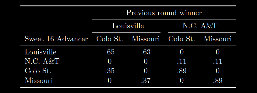
Here, the entries in the rows tell us how likely it is for a given team to advance, given the outcomes of the two games.  So, the .65 in the first line tell us that if Louisville and Colorado St. are victorious in the first round (and thus end up playing one another for the Sweet 16 slot), the probability that Louisville advances is 65%.  Contrastingly, the .35 in the third row tells us the probability of Colo. St. advancing (given Colorado St plays Louisville) is only 35%.  These percentages come from the "Probability of Victory" Bayesian model, that I explained in the last section.  Note that the probability of N.C. A&T or Missouri advancing to the Sweet 16 is zero in the first column.  This is because, if Louisville and Colorado State are playing for the Sweet 16 slot, then both N.C. A&T and Missouri have already been eliminated, and therefore, (obviously) cannot advance.  The other columns consider the other possibilities for the results of the previous games (e.g. column two considers that Louisville and Missouri won in the previous round).

Similar, but more complicated, conditional probability matrices are defined for all the other states in the tournament.  For example, each Final Four node has a matrix with 16 rows and 8x8=64 columns, because there are 16 possible teams that could occupy any given Final Four spot and there are 8 possible teams that could occupy each of the immediately proceeding Elite Eight spots.

Thus, a Bayesian model of the tournament in this manner allows us to efficiently consider all possible "what-if" scenarios of the tournament!

I built the Bayesian model of the tournament, and all of the conditional probabilities matrices, programatically, as I was not keen to specify the 64x32x32 = 65,536 entries required for the Championship node by hand!  For that I used the SMILE library, which is the programming library counterpart to the aforementioned GeNIe program.

Predictions and Selecting the Bracket

The above two models enabled explicit calculation of the probability that each team reaches each round of the tournament.  Shown below is a summary of these probabilities for the 10 teams my method predicts to be most likely to win the overall championship:

I thought predicting the tournament would be straightforward using this information, but there seems to be some subtlety here.  Suppose you start assigning the results in the 2nd round, then proceed to the Sweet 16 when that is finished, then to the Elite Eight, etc., choosing the team most likely to reach each of those nodes in turn.  Will that produce the optimal bracket?  I thought so!

However, consider this scenario: you have four teams.  Two of them are excellent, called QuiteGood and AlsoGood.  If they play each other, it's usually a pretty even game, but QuiteGood wins 51% of the time.  There are two other teams: Decent and Terrible.  Terrible essentially always loses (99% of the time).  If Decent plays either of QuiteGood or AlsoGood, Decent wins only 40% of the time, and loses 60% of the time.  So consider this bracket seeding:

The most likely outcome is that QuiteGood and Decent prevail in the first round and then QuiteGood wins the championship. Or, graphically:

So, this is the most likely bracket, therefore QuiteGood is the most likely to win the tournament, right?

No!  QuiteGood only plays in the championship 51% of the time and of that 51%, they only win 60% of the time.  Thus, their total probability of winning the championship is .51*.60 = .306 = 30.6%.  By contrast, Decent almost always gets to play in the championship game, and wins 40% of the time.  So Decent's probability of winning the tournament is 39.6%!  So Decent is the most likely winner of the tournament.

Since most scoring systems give greater weight to later games, predicting the champion with as much accuracy as possible is important.

Thus, in this simple scenario, the optimal bracket is not equivalent to the most likely bracket.  The optimal bracket is:

Obviously, the tournament seeding system is designed to avoid this scenario (i.e. good teams playing each other early), but that's no reason to rely on the tournament designers!  Indeed, if they were so good at correctly choosing seeds, perhaps we needn't even run a tournament at all!  Clearly, we should keep our own counsel about which teams are good.

Anyway, the practical result from this thought experiment is that calculating the bracket should proceed backwards.  Choose the tournament champion first, then the teams who reach the championship game, then the teams who reach the Final Four, etc.  In each case, I calculated my bracket by choosing the team with maximum probability to reach the furthest current round, working backward, but skipping teams when there was some bracketological impossibility.  For example, both Louisville (#1 in Midwest) and Duke (#2 in Midwest) cannot both reach the Final Four due to the structure of the tournament.  Thus Duke would have to be selected in an earlier round in the tournament (e.g. the Elite Eight), but that would be dealt with after assigning the Final Four round selections.

Downloads

Using this procedure, I obtained a final bracket, available by clicking here!

Additionally, you can feel free to look at my predictions for tournament survival probabilities, by clicking here!

EigenBracket 2012: Using Graph Theory to Predict NCAA March Madness Basketball

Last year one of the research associates in my lab asked if I wanted to make a bracket for the NCAA March Madness tournament.  Since I don't follow sports (other than what Jenny's interest in K-State sports exposes me to), I thought I wouldn't do very well just quasi-randomly picking teams.  Instead, I thought it would be a lot more fun to perform a mathematical analysis on the Win-Loss records for all the teams and use that data to "rationally" choose the bracket.

Last year, I had mixed results.  On the positive side, my bracket out-competed the members of my lab.  However, in the NCAA bracket group my family ran, my mom - who I am pretty sure made rather random choices - beat my bracket.

This year, I'm hoping to improve on that (limited) success.  Here's my strategy:

One of the most basic statistics about a team is their win-loss record.  For example, this year Kansas State had a win-loss record of 21-10.  Intuitively, we expect teams with favorable win-loss records to beat those with poor win-loss records.

Win-Loss record isn't the whole story, though, because all wins are not created equal.  Defeating a bad team is easy (and tells us very little), but defeating a good team is indicative of skill.  Therefore, a simple (though recursive) definition of a good team is: a team that is capable of winning games against other good teams.
 
Our major project, then, is to identify good teams without any a priori knowledge of team quality.
To find these teams, I modeled the win-loss history as a weighted, directed network.  To do this, I analyzed 5242 games played between Division I teams in the 2011-2012 season.

Win-loss history is simply a list of game results (e.g. K-State beat the Charleston South 72-67, then beat Loyola 74-61, then ... lost to West Virginia 80-85, ... etc).  A directed network is simply a connection of nodes (representing teams) and arrows connecting teams called directed edges.  Every time a team defeated another, an arrow was drawn from the losing team's node to the winning team's node to represent this game.

Note though that all wins are not created equal.  A game decided by a 20-point margin ("nuked from orbit", as I always say) is a lot different than a game decided by a single point.  In the former case, one team is clearly superior, while in the latter, the teams are roughly equal.  So let's revise our definition of a good team to be: a team that is capable of winning games against other good teams, by a large margin.

To account for this, each arrow is weighted between 0 and 1 to describe the magnitude of the victory.  Winning a game by a large margin results in an arrow with weight 1 being drawn from the loser to the winner.  By contrast, for games that are decided by only a few points, we'll draw arrows from both loser to winner AND winner to loser, both being weighted about 0.5 (slightly less for the loser).

Mathematically, edge weights can be calculated by using a a logistic function centered at zero.  We'll need to choose an operational definition of "winning by a large margin" (which corresponds to choosing how large a margin is required before a score of 0.9 is assigned to an edge).  Some experimentation (guided by a tiny amount of intuition) suggests that about 6 points is enough to definitively resolve that one team is better than another.

To find good teams, I computed each team's eigenvector centrality in the network.  For those who like math (if not, skip ahead to the next paragraph): any network can be modeled as an adjacency matrix.  The dominant eigenvector of this can be found by using power iteration.  The score assigned to the team associated with the i'th row of the adjacency matrix is given by the i'th element of the dominant eigenvector.

A simplified (and mostly accurate) way to think about this is that every team starts out with an equal number of "quality points".  Every time the computer says "Go", teams distribute their quality points to all the teams that beat them.  Thus, good teams get more quality points than they gave away (and vice versa for bad teams).  After a few rounds of this procedure, the quality points for every team approaches convergence.

[ Detail note: to prevent all the quality points from getting totally absorbed by undefeated [or nearly-so] teams, every team gives a small fraction of their points to every other team, just to keep some points in circulation. ]

Using this procedure, we can get a list of teams ranked in order of quality.

The top 10 ranked teams are (in order):

1. Kentucky
2. North Carolina
3. Syracuse
4. Missouri
5. Michigan St.
6. Ohio St.
7. Belmont
8. VCU
9. Kansas
10. Louisville

Note that the top 5 teams are all #1 or #2 seeded teams, but the algorithm did not know that a priori.  This provides a high-level validation to the algorithm.  Some other teams are seeded much lower.  For example, Belmont is a #14 seed, but has been talked about as an upset risk in their first game against Georgetown.  [ My analysis apparently does not think much of Georgetown, assigning it a rank of 65, which is in stark contrast to its #3 seed status ].

If you were wondering, the 5 lowest-scoring Division I teams - according to this particular analysis anyway - are (getting worse as you read down the list):

1. Fairleigh Dickinson
2. Binghamton
3. Tenn-Martin
4. Towson
5. Nebraska - Omaha

All of these teams have bad win-loss ratios except Nebraska-Omaha.  Looking at their record, it seems Nebraska-Omaha played a large number of Division II (?) teams, which are not included in the analysis.  Because there is some dependence on overall number of games played (which cancels out for most teams, because most play ~ 30 Division I games), this probably artificially makes their score low, which highlights a (minor) limitation of the algorithm.

If you're wondering where your favorite team is ranked, you can download the full ranked list:

Using this, we can predict the NCAA Tournament bracket using the simple heuristic that teams with higher eigenvector centrality rank ("more quality points") beat those with lower rank.  This produces what I call the Eigenbracket for the 2012 NCAA tournament.

The ultimate test of the bracket will be - of course - how well it predicts the tournament outcomes.  I tried to estimate the accuracy of my ranking method by using it to predict the results of all games across the whole season between either (a) all teams or (b) the top 80 teams.  In both cases, the accuracy was around 75%.

This isn't the best testing methodology because the test data is also being used to build the network.  A better way to test is to leave some data out (say, 10% of all games played), re-build the network and use those results to predict the outcomes of the games we held in reserve.  I experimented with this a a bit and think the results are similar (70-80% accuracy).  This also seems to do a little better than an analysis that fails to take into account margin of victory.  That strategy had about 65-75% accuracy.

In summary, network analysis can be applied to interesting problems to help make sense of huge datasets so that we can make informed predictions about the future.