Tuesday, March 25, 2014

Artificial Intelligence for 2048

I've always wanted to write an artificial intelligence (AI) that plays a video game by actually "watching" the screen and actually sending the right keyboard commands.  Today, I've done that for 2048, a sliding-tile game implemented in Javascript by Gabriele Cirulli.

In brief, you are given a 4x4 grid and must input UP, DOWN, LEFT or RIGHT to slide tiles.  Tiles move as far as they can go and when two tiles with the same number collide, they merge into a new tile with double the value of the original tiles.  When a key is pressed every tile moves, so every move impacts the entire board.  After every move, a new tile appears on the grid at a random location (a "2" tile with 90% probability or a "4" tile with 10% probability).  (If that was unclear, just play the game for a minute).  The objective is to merge tiles until the 2048 tile appears, which is a formidable challenge.  When the board is full and no moves can be made, the game is over.

I implemented a 2048 AI agent in C# that uses the Minimax algorithm with Alpha-Beta pruning to perform a local search of the game space.

When the software is launched, it estimates the location of the 2048 grid on the screen by looking for the leftmost pixel with the color of the exterior grid (R=187, G=173, B=160) and assumes the grid is 500x500 pixels.  After it finds the grid, it pauses to allow you to set your browser to the active window and then enters a loop.  Within the loop, it:

  1. Estimates the current state of the game
  2. Performs the minimax search to a depth of 6 player moves
  3. Sends the appropriate keypress to 2048 in the browser
  4. Wait a second for the 2048 animation to resolve (otherwise state estimation will be wrong)
State estimation uses the distinctive colors of the tiles (parsed out of the CSS file at http://gabrielecirulli.github.io/2048/style/main.css) to determine which tile occupies each space.  Colors are sampled in the upper-left corner of each tile, to avoid conflicting with the number.

By choosing the minimax algorithm, the AI treats 2048 as if it were a two-player game.  The first player is simply "the player" (the agent) and the second "player" is the random tile placement.  The AI assumes that the random tile placement will be chosen in the worst possible place (from the perspective of the AI).  Obviously, sometimes the (random!) placement won't always be worst-case, but by making this assumption, riskier lines of gameplay can be avoided.

Since minimax can only feasibly look-ahead several moves, the quality of the farthest states it can look at must be estimated.  I've used a very simple heuristic.  The quality of a state is equal to:

Quality = - [ (Number of occupied tiles) + Entropy/ln(16) ]

In general, it tries to minimize the number of tiles on the board.  The Entropy term is just the Shannon entropy of the distribution of non-zero tiles on the grid.  In simple terms, the entropy term just says "Prefer to have tiles of a few types, rather than of many types".  The idea is that it's easier to combine tiles if you have a grid of three "4"s than if you have a grid with one "4", one "8" and one "16".  The entropy term is scaled to be in the range of 0.0-1.0 so that minimizing the number of occupied tiles in the grid is the dominant guiding force.

Keypresses are sent using the Windows.System.Forms.SendKey API, which is incredibly convenient.  However, you'll need to use an implementation of C# that allows this.  This works on Windows, but I'm not sure if it will work on Linux under Mono (possibly, but I haven't tried it).

Overall, the AI tends to do pretty well when playing the game.  It does not always win, but if often does.

Software is implemented in C# and is available on GibHub at: https://github.com/djparente/AI2048

Please feel free to leave feedback in the comments!

Friday, February 28, 2014

PubMed BibTex QuickLink: A GreaseMonkey / TamperMonkey script adding a link to TexMed from PubMed

I have been writing my doctoral dissertation in LaTeX and have found TexMed -- a webserver that can provide the BibTex-formatted citation for any article in PubMed -- to be an invaluable resource.  My typical workflow has been:

  1. Find the article I want to cite on PubMed
  2. Copy the PubMed ID
  3. Search TexMed for the Pubmed ID
  4. Download the citation from TexMed
This works, but I'd rather cut out the middle steps.  So, I've written a script for Google Chrome* and Mozilla Firefox* that adds a new "[Get BibTex]" link to the PubMed pages that will directly take you to a TexMed page with the citation (screenshot below):


The script is available at UserScripts.org: http://userscripts.org/scripts/show/400556

UPDATE: As it looks like UserScripts.org is persistently down, the script is now available on GitHub: https://github.com/djparente/pubmed-texmed-quicklink as pubmed-bibtex-quicklink.js

*These work via the TamperMonkey and GreaseMonkey add-ins, respectively.

Tuesday, February 11, 2014

English word frequency list

I recently found myself in need of a English word list ordered by frequency, but could not find a free (in both freedom-of-use and free-of-charge senses) one that satisfied me.  So, I have compiled one using word counts in the Google Ngrams database, doing just a little processing to extract counts since 2005 (to avoid archaic words) and to strip out parts of speech identifiers from the word stems.

It seems adequate for my purposes, but have not done any extensive checking on it.  It should be adequate for common use ("Hello, how is your dog?"), but also for more formal writing.  For example, it contains the words "phylogenetic", "immunoblotting" and "histochemical" -- all fairly specialized molecular biology terms.

Be aware that there is no filtration on the terms included (i.e. if you want to strip out, e.g. profanity, you will need to do some further processing).  The file contains a header; these comments can be filtered out by excluding lines beginning with "#".  All entries are in lower case.

If this would be useful to you, the word list of the top 100,000 most common terms can be downloaded at: http://www.biophysengr.net/files/blog/wordlist/top100k_words_ngrams_djp.txt

The Ngrams data seems to be under Creative Commons Attribution 3.0 Unported license (CC-BY-3.0),  so I will follow suit for my processing of this list as well.

Happy word frequency-ing

Thursday, March 21, 2013

BayesianBracket 2013: A Bayesian Statistics Approach to Predicting NCAA March Madness Basketball

Last year, I wrote about predicting the NCAA Men's Basketball Tournament using graph theory to analyze the season's Win/Loss record network, thus creating the EigenBracket.  This year, I thought I'd try a new approach with three major ideas:
  1. Using player statistics of fundamentals (e.g. rebounds per game) to predict outcomes of games.
  2. Trying to assign a probability of victory, rather than just a "X team wins" result.
  3. Reasoning about the structure of the tournament itself (i.e. a #1 seed has an easier path to the championship than a #14 seed).

Player statistics

Last year, I had a lot of discussion with people about whether my model could account for late-season roster changes (e.g. last year I think there was a late change to the BYU roster).  In short, my EigenBracket model could not account for those effects.  To remedy that, I tried to include an explicit representation of players in the model this year, by looking at their individual statistics, including per game field goals, three pointers, free throws, rebounds, total points, assists, turnovers, steals, blocks and fouls.  To summarize these parameters for an entire team, I took the weighted average of individual statistics, weighting on the average playtime per game of each player.  The idea was that, in the event of a late-season roster change, that I could remove that player from the weighted average to model the impact on the team.
 
Armed with these summarized statistics, I set out to see if I could predict game outcomes using them (with Win-Loss data too, as I did last year).

Probability of Victory


Determining the probability of a victory of Team X over Team Y is most easily accomplished by training a statistical model.  One convenient method of doing this is to build a Bayesian model.  In short, these models are helpful when reasoning probabilistically about some hidden variable (will a team achieve victory) given a set of observations.

Every variable ("node") in the model has a finite set of states (e.g. True, False, etc.).  Nodes are connected by directed interconnections, called edges.  Edges between nodes essentially means "if the state of the (parent) variable is known, then I know something about the state of this other (child) variable."

For example, if you had your eyes closed while your favorite team was shooting a game-deciding free throw on the home court, you could still infer (probabilistically) whether the basket went in, based only on listening to whether the person next to you started cheering.  (But, this wouldn't tell you with certainty; your seat-neighbor might be a fan of the other team.  Nevertheless, it does update your belief in whether the basket was scored).  Thus, the [True, False] states of the Cheering variable, update your belief about the BasketScored state [Yes, No] and we would draw an edge between these variables.

I divided observations into two categories: those based on Win-Loss history and those based on player statistics:
  • For the Win-Loss history, I essentially calculated an ELO rating for each team.  I considered using the Eigenvector Centrality score from last year, but - since it was highly correlated with ELO scores anyway - thought a single feature was sufficient.
  • For Fundamentals, I used player statistics: per game field goals, three pointers, free throws, rebounds, total points, assists, turnovers, steals, blocks and fouls.
For any pair of teams (say, X and Y), the ELO and fundamental statistics can be characterized as Higher, Slightly Higher, Slightly Lower or Lower in team X, relative to team Y.  These can be entered as evidence in a model and the probability of victory (for team X) can be assigned.  To combine the ELO-based and Fundamentals-based predictors, I created two additional hidden variable nodes with three states: [Predict a Win, Predict a Loss, Indeterminate].  The rationale is that when teams with nearly equivalent ELO scores play each other, that ELO might be a bad predictor.  In that case, the ELO score could be set to Indeterminate by the model and Fundamentals could instead be used by the model to predict the outcome.  N.B.: I am not entirely sure if this behavior was fully realized in the trained model, but it was the rationale, nevertheless.


The full model is shown below, the available states of each node is shown in brackets:

Bayesian model used for calculating the probability of victory given two team's Win-Loss history and aggregate player statistics.
Overall, this model has about 75% accuracy on a random (validation) sample of 2012-2013 regular season games.  It's OK, but not perfect.

The thickness of the edge is related to the "strength of influence".  Thus, Win-Loss history (ELO scores) seem to be more predictive of victory than Fundamentals.  Amongst fundamentals, offensive parameters (Field Goals per game, etc) and Rebounds seem to be more predictive than defensive parameters (blocks, steals) or fouls.

But those conclusions should be taken with a grain of salt: I think the Fundamentals predictor is pretty weak.  Most of the predictive power of the model seems to come from Win-Loss data.  If the ELO node is removed from the model, a lot of the predictive power is lost.

For model building, and for prediction, I used the fantastic GeNIe bayesian analysis software from the University of Pittsburgh's Decisions Systems Laboratory. 

Structure of the Tournament


Actually, it turns out that using a Bayesian network is also a great way of modeling the tournament itself.  If every game is seen as having a probabilistic outcome (i.e. "Team X would beat Team Y nine times out of ten, on a neutral field"), the probability of each team reaching a given round can be explicitly modeled.  The Bayesian network actually has the same familiar form of a tournament bracket:


Subset of the full tournament Bayesian network (shown: upper part of the Midwest region bracket)

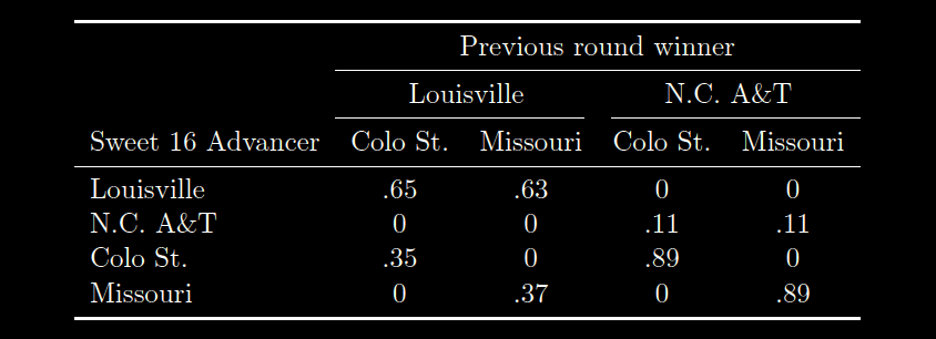
Each node in the tournament has a set of states that describe each of the possible teams that can reach that node.  For example, the uppermost Sweet 16 bracket in the Midwest region is reachable by four teams: Louisville, N.C. A&T, Colorado State and Missouri.  Thus, the node in the network representing the team reading the Sweet 16 from that part of the bracket has four states (each team).  Using Bayesian algorithms, we can calculate a vector of numbers describing how likely each of those states are (and, therefore, how likely each team is to reach the Sweet 16).  That vector doesn't have to be specified by the user; instead, it is calculated and depends on the vectors of the games immediately preceding it.  In this year's tournament, that means that the Upper-Midwest Sweet 16 node depends on the outcome of the Louisville vs N.C. A&T game, as well as the Colorado State vs Missouri game.  Thus, we can specify a conditional probability matrix for that Sweet 16 node, as follows:


Here, the entries in the rows tell us how likely it is for a given team to advance, given the outcomes of the two games.  So, the .65 in the first line tell us that if Louisville and Colorado St. are victorious in the first round (and thus end up playing one another for the Sweet 16 slot), the probability that Louisville advances is 65%.  Contrastingly, the .35 in the third row tells us the probability of Colo. St. advancing (given Colorado St plays Louisville) is only 35%.  These percentages come from the "Probability of Victory" Bayesian model, that I explained in the last section.  Note that the probability of N.C. A&T or Missouri advancing to the Sweet 16 is zero in the first column.  This is because, if Louisville and Colorado State are playing for the Sweet 16 slot, then both N.C. A&T and Missouri have already been eliminated, and therefore, (obviously) cannot advance.  The other columns consider the other possibilities for the results of the previous games (e.g. column two considers that Louisville and Missouri won in the previous round).

Similar, but more complicated, conditional probability matrices are defined for all the other states in the tournament.  For example, each Final Four node has a matrix with 16 rows and 8x8=64 columns, because there are 16 possible teams that could occupy any given Final Four spot and there are 8 possible teams that could occupy each of the immediately proceeding Elite Eight spots.

Thus, a Bayesian model of the tournament in this manner allows us to efficiently consider all possible "what-if" scenarios of the tournament!

I built the Bayesian model of the tournament, and all of the conditional probabilities matrices, programatically, as I was not keen to specify the 64x32x32 = 65,536 entries required for the Championship node by hand!  For that I used the SMILE library, which is the programming library counterpart to the aforementioned GeNIe program.

Predictions and Selecting the Bracket

The above two models enabled explicit calculation of the probability that each team reaches each round of the tournament.  Shown below is a summary of these probabilities for the 10 teams my method predicts to be most likely to win the overall championship:


I thought predicting the tournament would be straightforward using this information, but there seems to be some subtlety here.  Suppose you start assigning the results in the 2nd round, then proceed to the Sweet 16 when that is finished, then to the Elite Eight, etc., choosing the team most likely to reach each of those nodes in turn.  Will that produce the optimal bracket?  I thought so!

However, consider this scenario: you have four teams.  Two of them are excellent, called QuiteGood and AlsoGood.  If they play each other, it's usually a pretty even game, but QuiteGood wins 51% of the time.  There are two other teams: Decent and Terrible.  Terrible essentially always loses (99% of the time).  If Decent plays either of QuiteGood or AlsoGood, Decent wins only 40% of the time, and loses 60% of the time.  So consider this bracket seeding:

The most likely outcome is that QuiteGood and Decent prevail in the first round and then QuiteGood wins the championship. Or, graphically:
So, this is the most likely bracket, therefore QuiteGood is the most likely to win the tournament, right?

No!  QuiteGood only plays in the championship 51% of the time and of that 51%, they only win 60% of the time.  Thus, their total probability of winning the championship is .51*.60 = .306 = 30.6%.  By contrast, Decent almost always gets to play in the championship game, and wins 40% of the time.  So Decent's probability of winning the tournament is 39.6%!  So Decent is the most likely winner of the tournament.

Since most scoring systems give greater weight to later games, predicting the champion with as much accuracy as possible is important.

Thus, in this simple scenario, the optimal bracket is not equivalent to the most likely bracket.  The optimal bracket is:

Obviously, the tournament seeding system is designed to avoid this scenario (i.e. good teams playing each other early), but that's no reason to rely on the tournament designers!  Indeed, if they were so good at correctly choosing seeds, perhaps we needn't even run a tournament at all!  Clearly, we should keep our own counsel about which teams are good.

Anyway, the practical result from this thought experiment is that calculating the bracket should proceed backwards.  Choose the tournament champion first, then the teams who reach the championship game, then the teams who reach the Final Four, etc.  In each case, I calculated my bracket by choosing the team with maximum probability to reach the furthest current round, working backward, but skipping teams when there was some bracketological impossibility.  For example, both Louisville (#1 in Midwest) and Duke (#2 in Midwest) cannot both reach the Final Four due to the structure of the tournament.  Thus Duke would have to be selected in an earlier round in the tournament (e.g. the Elite Eight), but that would be dealt with after assigning the Final Four round selections.

Downloads


Using this procedure, I obtained a final bracket, available by clicking here!

Additionally, you can feel free to look at my predictions for tournament survival probabilities, by clicking here!

Saturday, July 28, 2012

Tutorial: Refraction in PovRay

I'm been experimenting with PovRay, a 3D ray tracing program based on constructive geometry.  Creating an image requires declaring a scene in a text file, not that dissimilar from writing a computer program.  When I was a kid, I remember my father teaching me about refraction by putting a pencil in a glass of water.  The pencil appears to bend because the path taken by photons reflected by the pencil bends via refraction - governed by Snell's law - then the pencil meets the water surface.  The water has an index of refraction (IOR) of about 1.3, while air is about 1.0.

Today, I'll show you how to simulate this effect in PovRay.  Please feel free to adapt the ideas present here into your own work (I'd appreciate it if you'd like to my blog though - but you don't have to).

If you don't already have PovRay installed you can get it here: http://www.povray.org/download/  Actually, as of this writing (2012-07-28), I recommend the version 3.7 release candidate: http://www.povray.org/beta/

Here is the final scene we will render (3840x2160 with 0.3 anti-aliasing; click to view full resolution):


Another view of the scene, showing the refraction more clearly from the side (click to view full resolution):


Our scene will include four objects:
  1. A partially transparent glass (index of refraction 1.5)
  2. Water (index of refraction 1.3)
  3. A straw
  4. A partially reflective surface for the glass to stand on

First, though, some setup parameters:


// Daniel J. Parente
// Licensed under CC 3.0-BY-SA

//Always use a version directive! 
//You might need to change this is you are using PovRay 3.6
#version 3.7;  

//Include some files
#include "colors.inc"
#include "textures.inc"
#include "glass.inc"

global_settings
{
   assumed_gamma 1.0   //For PovRay 3.7 (ver. 3.6 used 1.7, I think)
}
        
//Declare a constant to control the size of our glass
#declare BEAKER_HEIGHT=15;


//Declare a light source off to the left of the camera
light_source
{
   <0,20,-30>*3 color 1  //Same vector as the camera
   rotate 50*y           //Rotate off to the left
}   

camera
{
   location <0, 20, -30>*1.2         //Define a camera location
   up y                              //As usual, y is the up direction
   right image_width/image_height*x  //Configure the aspect ratio
   look_at <0, BEAKER_HEIGHT/3.5, 0> //Look at the middle of the beaker
}        

The glass


Then, we'll create the glass by constructing the difference of two cylinders: one with a slightly smaller radius and offset upward (the y direction) from the other.  We'll make the constructed object partially transparent, give it a glass finish and - importantly - configure the index of refraction:

//Define the glass beaker
difference
{
   cylinder
   {      
      //Main body of the cylinder
      <0,0,0>, <0, BEAKER_HEIGHT, 0>, 5
   }
   cylinder
   {      
      //Make it hollow (but offset in the y direction to give a bottom)
      //Hollow by creating another cylinder, a little thinner than the
      // outer cylinder
      <0,-5,0>, <0, BEAKER_HEIGHT+.1, 0>, 4.9
   }
   pigment
   {
      //Set the degree of transparency
      //(I think it ignores the R,G,B fields)
      rgbt .7
   }
   finish
   {
      //Look like glass
      Glass_Finish
   }      
   interior
   {
      ior 1.5  //Sets an index of refraction (1.5 is good for glass)
   }     
}

The water

The water is simply a partially transparent blue cylinder, with a radius that is slightly smaller than the glass's inner radius and with an index of refraction of 1.3

//Water            
cylinder
{
   //Define a cylinder just barely smaller (.05 units) than the beaker
   <0,1.0001,0>, <0, BEAKER_HEIGHT*.9, 0>, 4.85
   pigment
   {
      rgbt<0, 0, 1, .8>   //Blue, partially transparent
   }

   interior
   {
      ior 1.3 //Sets an index of refraction for water
   }
}  

The straw

To showcase the refraction, place a straw (a thin, hollowed-out cylinder) inside the glass of water:

//Create a straw
difference
{
   cylinder
   {      
      //Cylinder
      <0,0,0>, <0,BEAKER_HEIGHT*1.2,0>, .5
   }
  
   cylinder
   {
      //Slightly thinner, but longer cylinder to hollow it out
      <0,-1,0>, <0,BEAKER_HEIGHT*1.6,0>, .4
   }                
   finish
   {
      //Make it look a little like plastic
      phong .3
   }
   //Yellow color
   pigment{ rgb<255,240, 113>/255 }
  
   //Rotate it so it tilts a bit (and we can see the IOR effect)
   rotate 20*z
   rotate -20*x
  
   //Shift the straw into the water cylinder
   translate <2,BEAKER_HEIGHT/5, 2.5>
}  

The mirror plane


Lastly, we'll add a partially reflective "mirror" surface for the glass to sit on:

//Construct a mirror plane for the glass to sit on
plane
{
   <0,1,0>, -.001
   pigment
   {
      color White
   }            
      
   finish
   {      
      reflection .7
   }   
}

Rendering

Render the scene at 1920x1080 (or, whichever setting you choose, the aspect ratio should auto-adapt).  This took about 2 seconds on a hyper-threaded quad-core (14 CPU-seconds) using PovRay 3.7.0-RC6 for Windows 64-bit.

If you want to get a better look at the refraction, you can change the camera position to:

location <0, 10, -30>*1.2

This will produce the second, side-view image shown above.

I encourage you to vary some parameters in this scene (especially IOR values) to get a feel for how refraction works in PovRay.

You can download the full scene here: http://biophysengr.net/files/blog/povray/water_refraction.pov

Standard disclaimers and statements
I am not affiliated PovRay. I have not accepted compensation in any form from any organization in support of this project. Use this information at your own risk. I am not responsible for any adverse effects your use of this information causes. 

Wednesday, June 27, 2012

Writing sketches to a ATmega328 pre-loaded with the Arduino Uno bootloader using an Arduino Uno and ArduinoISP

Hopefully this post is not excessively redundant, but I had difficulty finding clear instructions on the Internet on how to:

Upload a new sketch to a standalone ATmega328 (pre-loaded with an Arduino bootloader) using an existing Arduino Uno without removing the existing ATmega chip from my Uno.

This is useful because:
  • You won't need to buy an external AVR programmer (this method is very low cost!)
  • It doesn't require constant removal of the on-Arduino ATmega328 chip to "directly" use the Tx/Rx lines (because those pins will eventually break
I found several posts on how to program a standalone ATmega with a bootloader (for example, the main ArduinoISP page), but those pages typically did not discuss uploading sketches using ArduinoISP.  I did find one page suggesting a (complicated) method of doing this by modifying boards.txt, though I did not have success using that method.

Anyway, some trial and error over the course of an hour or so revealed that uploading sketches to an external ATmega is very simple.  For this, you will need:
  • An Arduino Uno (mine is rev 3)
  • An ATmega328 microprocessor pre-loaded with Arduino bootloader (I bought this one, preloaded with the Uno optiboot bootloader, from Sparkfun).
  • A 16 MHz crystal oscillator
  • Two 22 pF ceramic capacitors
  • A 10 kOhm resistor
  • A capacitor with capacitance > 10 uF (I used a 22 uF capacitor, but others have reported success with  10 uF capacitors).
First, wire up the external ATmega circuitry:
  • Pins 7 and 20 to +5V
  • Pins 8 and 22 to Gnd
  • Pin 1 (reset) to +5V through a 10 kOhm resistor
  • Crystal oscillator to pins Z and K
  • A 22 pF capacitor connecting each pin of the oscillator to ground
A good diagram is found here: http://www.jameco.com/Jameco/workshop/JamecoBuilds/arduinocircuit.html (Note: those instructions also connect pin 21 [AREF] to Gnd, but I did not do so when I tried this).

Next, connect your Arduino Uno to the USB port of your computer, open up Arduino IDE (version 1.0.1 or later), select the ArduinoISP sketch from the examples file (see image below) and upload this to your Arduino like you would any other sketch.

How to find the ArduinoISP sketch

Now disconnect your Uno from the USB port (thereby disconnecting power) and wire the following connections:
  • Arduino pin 10 to Standalone Pin 1 [Reset]
  • Arduino pin 11 to Standalone Pin 17
  • Arduino pin 12 to Standalone Pin 18
  • Arduino pin 13 to Standalone Pin 19
Make sure you also supply power to the breadboard by connecting the 5V and Gnd pins on the Arduino board to the breadboard power supply rails.  The final circuit is the same as the one on the ArduinoISP page (i.e. using an external circuit); image here: http://arduino.cc/en/uploads/Tutorial/BreadboardAVR.png

If your arduino auto-resets when a serial connection is established (e.g. when you load a new program), you will need to disable it.  There is a page describing this, but for my Uno, the simplest solution was to put a 22 uF capacitor between the reset and Gnd pins.  Others have reported success with other capacitor values; the most common value I have seen is 10 uF.

Your Arduino is now ready to act as a programmer for the standalone ATmega chip.  Plug it back into the USB port.  Load the sketch you want to program the standalone ATmega chip with into the Arduino IDE (I recommend "blink" while you are trying this out for the first time).  Set the IDE to use the programmer "Arduino as ISP" as in the image below:

Configure Arduino IDE to use the connected Arduino as an ISP

Then upload the sketch using the programmer:

Upload your sketch using the connected (ArduinoISP) programmer

The Rx/Tx lines should flash for a few seconds on your Arduino board.  When it finishes, your standalone ATmega should be programmed with the desired sketch.  The Arduino will continue to be programmed with the ArduinoISP sketch.

Disconnect power (the USB plug) from both circuits and remove the jumpers between the Arduino and the standalone ATmega chip.  Remove the 22 uF capacitor between the Reset/Gnd pins on your Arduino to return it back to a state where you can re-program it away from the ArduinoISP state.

Hopefully, you now know how to program an external ATmega chip by (completely reversibly!) converting your Arduino to an ISP.  Please feel free to leave comments if (a) this worked for you, (b) this didn't work for you and tell us what you're seeing, or (c) if you've noticed any mistakes in my instructions (though I have striven to eliminate errors).

Standard disclaimers and statements
I am not affiliated Arduino or any of the retailers mentioned above.  I have not accepted compensation in any form from any organization in support of this project.  Use this information at your own risk as there is always a possibility of undetected inaccuracies.  I am not responsible for any adverse effects your use of this information causes including, but not limited to, damage to hardware or humans.

Tuesday, March 13, 2012

EigenBracket 2012: Using Graph Theory to Predict NCAA March Madness Basketball

Last year one of the research associates in my lab asked if I wanted to make a bracket for the NCAA March Madness tournament.  Since I don't follow sports (other than what Jenny's interest in K-State sports exposes me to), I thought I wouldn't do very well just quasi-randomly picking teams.  Instead, I thought it would be a lot more fun to perform a mathematical analysis on the Win-Loss records for all the teams and use that data to "rationally" choose the bracket.

Last year, I had mixed results.  On the positive side, my bracket out-competed the members of my lab.  However, in the NCAA bracket group my family ran, my mom - who I am pretty sure made rather random choices - beat my bracket.

This year, I'm hoping to improve on that (limited) success.  Here's my strategy:

One of the most basic statistics about a team is their win-loss record.  For example, this year Kansas State had a win-loss record of 21-10.  Intuitively, we expect teams with favorable win-loss records to beat those with poor win-loss records.

Win-Loss record isn't the whole story, though, because all wins are not created equal.  Defeating a bad team is easy (and tells us very little), but defeating a good team is indicative of skill.  Therefore, a simple (though recursive) definition of a good team is: a team that is capable of winning games against other good teams.
 
Our major project, then, is to identify good teams without any a priori knowledge of team quality.
To find these teams, I modeled the win-loss history as a weighted, directed network.  To do this, I analyzed 5242 games played between Division I teams in the 2011-2012 season.

Win-loss history is simply a list of game results (e.g. K-State beat the Charleston South 72-67, then beat Loyola 74-61, then ... lost to West Virginia 80-85, ... etc).  A directed network is simply a connection of nodes (representing teams) and arrows connecting teams called directed edges.  Every time a team defeated another, an arrow was drawn from the losing team's node to the winning team's node to represent this game.

Note though that all wins are not created equal.  A game decided by a 20-point margin ("nuked from orbit", as I always say) is a lot different than a game decided by a single point.  In the former case, one team is clearly superior, while in the latter, the teams are roughly equal.  So let's revise our definition of a good team to be: a team that is capable of winning games against other good teams, by a large margin.

To account for this, each arrow is weighted between 0 and 1 to describe the magnitude of the victory.  Winning a game by a large margin results in an arrow with weight 1 being drawn from the loser to the winner.  By contrast, for games that are decided by only a few points, we'll draw arrows from both loser to winner AND winner to loser, both being weighted about 0.5 (slightly less for the loser).

Mathematically, edge weights can be calculated by using a a logistic function centered at zero.  We'll need to choose an operational definition of "winning by a large margin" (which corresponds to choosing how large a margin is required before a score of 0.9 is assigned to an edge).  Some experimentation (guided by a tiny amount of intuition) suggests that about 6 points is enough to definitively resolve that one team is better than another.

To find good teams, I computed each team's eigenvector centrality in the network.  For those who like math (if not, skip ahead to the next paragraph): any network can be modeled as an adjacency matrix.  The dominant eigenvector of this can be found by using power iteration.  The score assigned to the team associated with the i'th row of the adjacency matrix is given by the i'th element of the dominant eigenvector.

A simplified (and mostly accurate) way to think about this is that every team starts out with an equal number of "quality points".  Every time the computer says "Go", teams distribute their quality points to all the teams that beat them.  Thus, good teams get more quality points than they gave away (and vice versa for bad teams).  After a few rounds of this procedure, the quality points for every team approaches convergence.

[ Detail note: to prevent all the quality points from getting totally absorbed by undefeated [or nearly-so] teams, every team gives a small fraction of their points to every other team, just to keep some points in circulation. ]

Using this procedure, we can get a list of teams ranked in order of quality.

The top 10 ranked teams are (in order):
  1. Kentucky
  2. North Carolina
  3. Syracuse
  4. Missouri
  5. Michigan St.
  6. Ohio St.
  7. Belmont
  8. VCU
  9. Kansas
  10. Louisville
Note that the top 5 teams are all #1 or #2 seeded teams, but the algorithm did not know that a priori.  This provides a high-level validation to the algorithm.  Some other teams are seeded much lower.  For example, Belmont is a #14 seed, but has been talked about as an upset risk in their first game against Georgetown.  [ My analysis apparently does not think much of Georgetown, assigning it a rank of 65, which is in stark contrast to its #3 seed status ].

If you were wondering, the 5 lowest-scoring Division I teams - according to this particular analysis anyway - are (getting worse as you read down the list):
  1. Fairleigh Dickinson
  2. Binghamton
  3. Tenn-Martin
  4. Towson
  5. Nebraska - Omaha
All of these teams have bad win-loss ratios except Nebraska-Omaha.  Looking at their record, it seems Nebraska-Omaha played a large number of Division II (?) teams, which are not included in the analysis.  Because there is some dependence on overall number of games played (which cancels out for most teams, because most play ~ 30 Division I games), this probably artificially makes their score low, which highlights a (minor) limitation of the algorithm.

If you're wondering where your favorite team is ranked, you can download the full ranked list:


Using this, we can predict the NCAA Tournament bracket using the simple heuristic that teams with higher eigenvector centrality rank ("more quality points") beat those with lower rank.  This produces what I call the Eigenbracket for the 2012 NCAA tournament.


The ultimate test of the bracket will be - of course - how well it predicts the tournament outcomes.  I tried to estimate the accuracy of my ranking method by using it to predict the results of all games across the whole season between either (a) all teams or (b) the top 80 teams.  In both cases, the accuracy was around 75%.

This isn't the best testing methodology because the test data is also being used to build the network.  A better way to test is to leave some data out (say, 10% of all games played), re-build the network and use those results to predict the outcomes of the games we held in reserve.  I experimented with this a a bit and think the results are similar (70-80% accuracy).  This also seems to do a little better than an analysis that fails to take into account margin of victory.  That strategy had about 65-75% accuracy.

In summary, network analysis can be applied to interesting problems to help make sense of huge datasets so that we can make informed predictions about the future.